《算法图解》阅读笔记
1. 算法简介
1.1. 引言
1.2. 二分查找
def binary_search(list, item):
    low = 0
    high = len(list)
    while low <= high:
        mid = int((low + high) / 2)
        mid_v = list[mid]
        if mid_v == item:
            return mid
        elif mid_v < item:
            low = mid + 1
        else:
            high = mid - 1
    return None

print(binary_search([1,4,5,7,8,33,333,445], 33))
1.3. 大O表示法
- 算法的运行时间是从其n增速的角度度量的
- 大O表示法指出了最糟糕情况下的运行时间
1.3.1. 常见的大O运行时间
- O(log2n)
- O(n)
- O(n * log2n)
- O(n2)
- O(n!) 旅行商人问题
2. 选择排序
2.1. 内存的工作原理
2.2. 数组和链表
| 数组 | 链表 | |
|---|---|---|
| 读取 | O(1) | O(n) |
| 插入 | O(n) | O(1) |
| 删除 | O(n) | O(1) |
2.3. 选择排序
时间复杂度 O(n2)
def findSmallest(arr):
    smallest = arr[0]
    smallest_idx = 0
    for i in range(1, len(arr)):
        if arr[i] < smallest:
            smallest_idx = i
            smallest = arr[i]
    return smallest_idx

def selectionSort(arr):
    result = []
    for i in range(len(arr)):
        smallest_idx = findSmallest(arr)
        result.append(arr.pop(smallest_idx))
    return result

print(selectionSort([1,5,3,1,3,5,7,4,3,2,4]))
print(selectionSort([1,5,3,345,23,12,3,4]))
3. 递归
3.1. 递归
3.2. 基线条件和递归条件
3.3. 栈
- 由于 调用栈 的存在,使用递归会占用大量的内存
- 可通过 尾递归 来优化
4. 快速排序
4.1. 分而治之
divide and conquer
- 找出简单的基线条件
- 确定如何缩小规模,使其符合基线条件
4.2. 快速排序
def quicksort(arr):
    if len(arr) < 2:
        return arr
    base = arr.pop()
    low_arr = []
    high_arr = []
    for i in arr:
        if i > base:
            high_arr.append(i)
        else:
            low_arr.append(i)
    return quicksort(low_arr) + [base] + quicksort(high_arr)

quicksort([1,2,33,43,3,9,2,3,1])
平均情况(最佳情况) O(n * log2n) 最差情况 O(n2)
4.3. 再谈大O表示法
5. 散列表
5.1. 散列函数
- 相同的输入,相同的输出
- 不同的输出,不同的输出
- 只返回有效的索引
散列表使用数组来储存数据
5.2. 应用案例
5.3. 冲突
解决冲突的一种方式:对于冲突的key, 其value 储存一个链表,链接的节点储存 K/V
5.4. 性能
| 散列表(平均) | 散列表(最差) | 数组 | 链表 | |
|---|---|---|---|---|
| 查找 | O(1) | O(n) | O(1) | O(n) |
| 插入 | O(1) | O(n) | O(n) | O(1) |
| 删除 | O(1) | O(n) | O(n) | O(1) |
减少冲突:
- 较小的填装因子
- 较好的散列函数
5.4.1. 填装因子
\begin{equation}
\frac{散列表包含的元素数}{位置总数}
\end{equation}
一旦填装因子大于0.7, 就该调整散列表的长度
6. 广度优先搜索
6.1. 图简介
6.2. 图是什么
- 图模拟一组链接
- 图由节点和边界组成
6.3. 广度优先搜索
广度优先搜索回答两类问题:
- 从节点A出发,有前往节点B的路径吗?
- 从节点A出发,前往节点B的哪条路径最短?
6.4. 实现图
- 可以用散列表实现图
- 有向图的边为箭头,箭头的方向确定了关系的方向
- 无向图的边不带箭头,其中关系是双向的
6.5. 实现算法
from collections import deque

graph = {}
graph['you'] = ['alice', 'bob', 'claire']
graph['alice'] = ['job', 'claire']
graph['claire'] = ['marry']
graph['marry'] = ['mark']

def is_seller(person):
    return person == 'mark'

search_queue = deque()
search_queue += graph['you']
print(graph)

def search(search_queue):
    searched = set()
    while search_queue:
        person = search_queue.popleft()
        if person in searched:
            continue
        searched.add(person)
        if is_seller(person):
            print('find seller')
            return True
        elif graph.get(person):
            search_queue += graph[person]
    return False

search(search_queue)
时间复杂度为 O(V+E) V为顶点数,E为边数. 执行了 E 次遍历 和 V 次添加队列操作
7. 狄克斯特拉算法
7.1. 使用狄克斯特拉算法
- 找出最便宜的节点
- 对于该节点的邻居,检查是否有前往它们的最短路径,如果有,就更新开销
- 重复该过程
- 计算最终路径
7.2. 术语
带权重的图称为加权图
7.3. 换钢琴
7.4. 负权边
狄克斯特拉算法假设的条件
- 没有负权边
- 对于处理过的节点,没有前往该节点的最短路径
对于有负权边的,可以使用 贝尔曼-福德算法
7.5. 实现
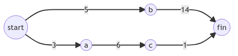
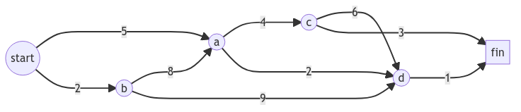
def find_lowest_cost_node(costs, processed):
    lowest_cost = float('inf')
    lowest_node = None
    for n in costs.keys():
        if n not in processed and costs[n] < lowest_cost:
            lowest_cost = costs[n]
            lowest_node = n
    return lowest_node


def find_lowest_path(graph):
    processed = set()
    costs = {}
    parents = {}
    for n in graph['start'].keys():
        costs[n] = graph['start'][n]
        parents[n] = 'start'
    node = find_lowest_cost_node(costs, processed)
    while node is not None:
        cost = costs[node]
        if node in graph:
            neighbors = graph[node]
            for n in neighbors.keys():
                new_cost = cost + neighbors[n]
                if n not in costs or costs[n] > new_cost:
                    costs[n] = new_cost
                    parents[n] = node
        processed.add(node)
        node = find_lowest_cost_node(costs, processed)
    print(costs['fin'])
    str = 'fin'
    parent = parents['fin']
    while parent in parents:
        str = parent + '->' + str
        parent = parents[parent]
    print('start->' + str)

graph = {}
graph['start'] = {}
graph['start']['a'] = 3
graph['start']['b'] = 5
graph['a'] = {}
graph['a']['c'] = 6
graph['b'] = {}
graph['b']['fin'] = 14
graph['c'] = {}
graph['c']['fin'] = 1
print(graph)
find_lowest_path(graph)

graph1 = {}
graph1['start'] = {}
graph1['start']['a'] = 5
graph1['start']['b'] = 2
graph1['b'] = {}
graph1['b']['a'] = 8
graph1['b']['d'] = 7
graph1['a'] = {}
graph1['a']['c'] = 4
graph1['a']['d'] = 2
graph1['c'] = {}
graph1['c']['d'] = 6
graph1['c']['fin'] = 3
graph1['d'] = {}
graph1['d']['fin'] = 1
print(graph1)
find_lowest_path(graph1)
时间复杂度 O(n2)
8. 贪婪算法
8.1. 教室调度问题
贪婪算法每步都采取局部最优解
贪婪算法并不一定是最优解,它是一种近似算法
8.2. 背包问题
8.3. 集合覆盖问题
stations = {}
stations["k1"] = {"id", "nv", "ut"}
stations["k2"] = {"wa", "id", "mt"}
stations["k3"] = {"or", "nv", "ca"}
stations["k4"] = {"nv", "ut"}
stations["k5"] = {"ca", "az"}

# 找出覆盖所有 states 的最小的集合,

def find_min(stations):
    result_stations = set()
    states_covered = set()

    while True:
        best_states = set()
        best_station = None
        for station, states in stations.items():
            if station not in result_stations:
                covered = states - states_covered
                if len(covered) > len(best_states):
                    best_states = covered
                    best_station = station
        if best_station == None:
            break
        result_stations.add(best_station)
        states_covered = states_covered | best_states
    return result_stations

print(find_min(stations))
8.4. NP完全问题
诸如 旅行商人问题 集合覆盖问题 ,需要计算所有的解,并从中选取最小的那个,以难解著称的问题。 这类问题一般采用近似求解